2.1 Introduction
What is probability?
- The first interpretation is called the frequentist interpretation. In this view, probabilities represent long run frequencies of events.
- The other interpretation is called the Bayesian interpretation of probability. In this view, probability is used to quantify our uncertainty about something; hence it is fundamentally related to information rather than repeated trials (Jaynes 2003).
2.2 A brief review of probability theory
- Discrete random variables (probability mass function, abbreviated to pmf)
- Fundamental rules, including Probability of a union of two events, Joint probabilities, Conditional probability
- Bayes rule: Combining the definition of conditional probability with the product and sum rules yields Bayes rule, also called Bayes Theorem:
- Independence and conditional independence
- X and Y are unconditionally independent or marginally independent:
- X and Y are conditionally independent (CI) given Z iff the conditional joint can be written as a product of conditional marginals:
\(X \perp Y|Z \Leftrightarrow p(X,Y|Z) = p(X|Z)p(Y|Z)\) Theorem 2.2.1.: $X\bot Y |Z$ iff there exist function $g$ and $h$ such that $p(x, y|z) = g(x, z)h(y, z) $ for all $x,y,z$ such that $p(z) > 0$.
(! Need to be proved)
- Continuous random variables(probability density function, abbreviated to pdf; cumulative distribution function, abbreviated to cdf)
- Quantiles: denoted by $F^−1(\alpha)$
- Mean(expected value), standard deviation and variance(a measure of the “spread” of a distribution)
2.3 Some common discrete distributions
- The binomial and Bernoulli distributions
-
binomial distribution $X \sim Bin(n,\theta)$:
\[Bin(k|n,\theta) \triangleq \binom{n}{k}\theta^k(1-\theta)^{n-k}\]where $\binom{n}{k} \triangleq \frac{n!}{k!(n-k)!}$ is the number of ways to choose k items from n (this is known as the binomial coefficient, and is pronounced “n choose k”).
-
Bernoulli distribution $X \sim Ber(\theta)$:
\(Ber(x|\theta) \triangleq \theta^{\mathbb{I}(x=1)}(1-\theta)^{\mathbb{I}(x=0)} = \begin{cases} \theta & \text{if x=1}\\ 1-\theta & \text{if x=0} \end{cases}\) Bernoulli distribution is the special case of a binomial distribution with $n=1$
binomial distribution: How many times(k) do the coin face up when it is thrown for n times?
Bernoulli distribution: Do the coin face up when it is thrown for once?
-
- The multinomial and multinoulli distributions
-
multinomial distributions: \(Mu(\pmb{x}|n, \pmb{\theta} ) \triangleq \binom{n}{x_1\cdots x_K}\prod_{j=1}^{K}\theta_j^{x_j}\)
where $\binom{n}{x_1\cdots x_K} \triangleq \frac{n!}{x_1!x_2!\cdots x_K!}$ is the multinomial coefficient and $\sum x_i = n$
-
multinoulli distributions(x is its dummy encoding or one-hot encoding): \(Cat(x|\pmb{\theta}) \triangleq Mu(\pmb{x}|1, \pmb{\theta} ) \triangleq \prod_{j=1}^{K}\theta_j^{\mathbb{I}(x_j=1)}\) This very common special case is known as a categorical or discrete distribution. And $p(x = j|\pmb{\theta}) = \theta_j$
multinomial distribution: How many times for each surface ( $[x_1\cdots x_6]$ ) do a dice show when it is thrown for n times?
multinoulli distribution: What surface do a dice show when it is thrown for once?
Name n K x mean variance Multinomial - - $x\in {0,1,\cdots, n}^K, \sum_{k=1}^{K}x_k=n$ $E(X_j) = n\theta_j$ $Var(X_j) = n\theta_j(1-\theta_j)$, $Cov(X_i, X_j) = -n\theta_i\theta_j$ Multinoulli 1 - $x\in {0,1}^K, \sum_{k=1}^{K}x_k=1$(1-of-K encoding) $E(X_j) = n\theta_j$ $Var(X_j) = \theta_j(1-\theta_j)$, $Cov(X_i, X_j) = -\theta_i\theta_j$ Binomial - 1 $x\in {0,1,\cdots, n}$ $\theta$ $n\theta(1-\theta)$ Bernoulli 1 1 $x\in {0,1}$ $\theta$ $\theta(1-\theta)$ -
-
The Poisson distribution \(Poi(x|\lambda) = e^{-\lambda}\frac{\lambda^x}{x!}\) The first term is just the normalization constant, required to ensure the distribution sums to 1.
-
The empirical distribution Given a set of data, $D = {x_1,\cdots,x_N}$, we define the empirical distribution, also called the empirical measure, as follows:
\[p_{emp}(A) \triangleq \frac{1}{N}\sum_{i=1}^N\delta_{x_i}(A)\]where $\delta_{x}(A)$ is the Dirac measure, defined by
\[\delta_{x}(A) = \begin{cases} 0 & \text{if } x \notin A\\ 1 & \text{if } x \in A \end{cases}\]PS: in my opinion, indicator function $\mathbb{I}_A(x)$ and Dirac measure $\delta_x(A)$ mean the same thing but their parameters are inversed.
In general, we can associate “weights” with each sample:
\[p(x) = \sum_{i=1}^Nw_i\delta_{x_i}(x)\]where it is required that $0\leq w_i\leq 1$ and $\sum w_i = 1$
According to Wiki,
In statistics, an empirical distribution function is the distribution function associated with the empirical measure of a sample. This cumulative distribution function is a step function that jumps up by $1/n$ at each of the $n$ data points.
2.4 Some common continuous distributions
-
Gaussian (normal) distribution
\[\mathcal{N}(x|\mu, \theta) \triangleq \frac{1}{\sqrt{2\pi\sigma^2}}e^{-\frac{1}{2\sigma^2}(x-\mu)^2}\]Here $\sqrt{2\pi\sigma^2}$ is the normalization constant needed to ensure the density integrates to 1.(!Need to be proved)
Standard normal distribution is sometimes called the bell curve.
We will often talk about the precision of a Gaussian, by which we mean the inverse variance: $\lambda = \frac{1}{σ^2}$.
Question: What’s the meaning of this sentence?
Note that, since this is a pdf, we can have $p(x) > 1$. To see this, consider evaluating the density at its center, $x = \mu$. We have $\mathcal{N}(\mu|\mu,\sigma^2) = (\sigma\sqrt{2\pi})^{−1}e^0$, so if $\sigma < 1/\sqrt{2\pi}$, we have $p(x) > 1$. Why does the author mention this?
The cumulative distribution function has no closed form expression but it can be calculated by error function(erf):
\[\Phi(x;\mu,\sigma)=\frac{1}{2}[1+erf(z/\sqrt{2})] \\ erf(x) \triangleq \frac{2}{\sqrt{\pi}}\int_0^xe^{-t^2}dt\]where $z=(x-\mu)/\sigma$.
Gaussian distribution is widely used because:
- it has two parameters which are easy to interpret
- the central limit theorem (Section 2.6.3) tells us that sums of independent random variables have an approximately Gaussian distribution (good for modeling errors or noise)
- Gaussian distribution makes the least number of assumptions (why?)
- simple mathematical form
-
Degenerate pdf In the limit that $\sigma^2 \rightarrow 0$, the Gaussian becomes an infinitely tall and infinitely thin “spike” centered at $\mu$
\[\lim_{\sigma^2 \rightarrow 0} \mathcal{N}(x|\mu,\sigma^2)=\delta(x-\mu)\]where $\delta$ is called a Dirac delta function, defined as:
\[\delta(x) = \begin{cases} \infty & \text{if } x=0\\ 0 & \text{if }x\neq 0 \end{cases}\]such that $\int_{-\infty}^{\infty}\delta(x)dx=1$
A useful property of delta functions is the sifting property, which selects out a single term from a sum or integral: \(\int_{-\infty}^{\infty}f(x)\delta(x-\mu)dx=f(\mu)\)
One problem with the Gaussian distribution is that it is sensitive to outliers (big change on $x$ results in bigger change on $e^{(x-\mu)^2}$)
Thus, A more robust distribution is the Student $t$ distribution:
\[\mathcal{T}(x|\mu,\sigma^2,\nu) \propto \Big[1+\frac{1}{\nu}(\frac{x-\mu}{\sigma})^2\Big]^{-\frac{\nu+1}{2}}\]where $\mu$ is the mean, $\sigma^2>0$ is the scale parameter and $\nu>0$ is the degrees of freedom. Its mean is $\mu$, mode is $\mu$,variance is $\frac{\nu\sigma^2}{(\nu-2)}$. The variance is only defined if $\nu > 2$. The mean is only defined if $\nu > 1$.
Because the Student has heavier tails, it hardly changes when adding some outliers. It is common to use $\nu = 4$ because of some good performance. But For $\nu \geq 5$, the Student distribution rapidly approaches a Gaussian distribution and loses its robustness properties.
-
The Laplace distribution (a.k.a. double sided exponential distribution)
\[Lap(x|\mu,b) \triangleq \frac{1}{2b}exp(-\frac{|x-\mu|}{b})\]Here $\mu$ is a location parameter and $b > 0$ is a scale parameter.
mean = $\mu$, mode = $\mu$, var = $2b^2$
It is also robust to outliers. It also put mores probability density at 0 than the Gaussian. This property is a useful way to encourage sparsity in a model (L1-regulation)
-
The gamma distribution The gamma distribution is a flexible distribution for positive real valued rv’s, $x > 0$. It is defined in terms of two parameters, called the shape $a > 0$ and the rate $b > 0$:
\[Ga(T|shape=a,rate=b) \triangleq \frac{b^a}{\Gamma(a)}T^{a-1}e^{-Tb}\]where $\Gamma(a)$ is the gamma function:
\[\Gamma(x) \triangleq \int_0^{\infty}u^{x-1}e^{-u}du\]mean = $a/b$, mode = $(a-1/b)$, var = $a/b^2$
Gamma Distribution is also widely used, such as:
- Exponential distribution: $Expon(x|\lambda) = Ga(x|1, \lambda)$
- Erlang distribution: a is an integer
- Chi-squared distribution: $\chi^2(x|\nu) = Ga(x|\nu,1)$
Besides, if $X \sim Ga(a,b)$, then $1/X \sim IG(a,b)$, where IG is the inverse gamma distribution.
mean = $b/(a-1)$, mode = $b/(a+1)$, var = $b^2/((a-1)^2(a-2))$
-
The beta distribution The beta distribution has support over the interval [0, 1] and is defined as follows:
\[Beta(x|a, b) = \frac{1}{B(a,b)} x^{a−1}(1 − x)^{b−1}\]where $B(a,b)$ is the beta function:
\[B(a,b) \triangleq \frac{\Gamma(a)\Gamma(b)}{\Gamma(a+b)}\]If $a = b = 1$, we get the uniform distirbution.
mean = $\frac{a}{b}$, mode = $\frac{a-1}{a+b-2}$, var = $\frac{ab}{(a+b)^2(a+b+1)}$
-
Pareto distribution The Pareto distribution is used to model the distribution of quantities that exhibit long tails, also called heavy tails. You may think of Pareto principle, which is called “二八原则” in Chinese.
\[Pareto(x|k, m) = km^kx^{−(k+1)}\mathbb{I}(x \geq m)\]If we plot the distibution on a log-log scale, it form a straight line, of the form $\log p(x) = a\log x + c$ (a.k.a. power law)
You can know more power law in 浅谈网络世界中的Power Law现象(一) 什么是Power Law
mean = $\frac{km}{k-1}$ if $k>1$, mode = $m$, var = $\frac{m^2k}{(k-1)^2(k-2)}$ if $k > 2$
2.5 Joint probability distributions
- Covariance and correlation
- Uncorrelated does not imply independent
- Independent does imply uncorrelated
- The multivariate Gaussian
-
The multivariate Gaussian or multivariate normal (MVN) is the most widely used joint probability density function for continuous variables.
\[\mathcal{N}(\pmb{x}|\pmb{\mu}, \pmb{\Sigma}) \triangleq \frac{1}{(2\pi)^{D/2}|\pmb{\Sigma}|^{1/2}}exp\Big[ -\frac{1}{2} (\pmb{x}-\pmb{\mu})^T\pmb{\Sigma}^{-1}(\pmb{x}-\pmb{\mu}) \Big]\]where $\mu = E[x] \in \mathbb{R}^D$ is the mean vector, and $\Sigma = cov[x]$ is the $D \times D$ covariance matrix. Sometimes we will work in terms of the precision matrix or concentration matrix instead. This is just the inverse covariance matrix, $\Lambda = \Sigma^{−1}$.
-
Multivariate Student $t$ distribution
A more robust alternative to the MVN is the multivariate Student t distribution. The smaller $\nu$ is, the fatter the tails.
-
Dirichlet distribution
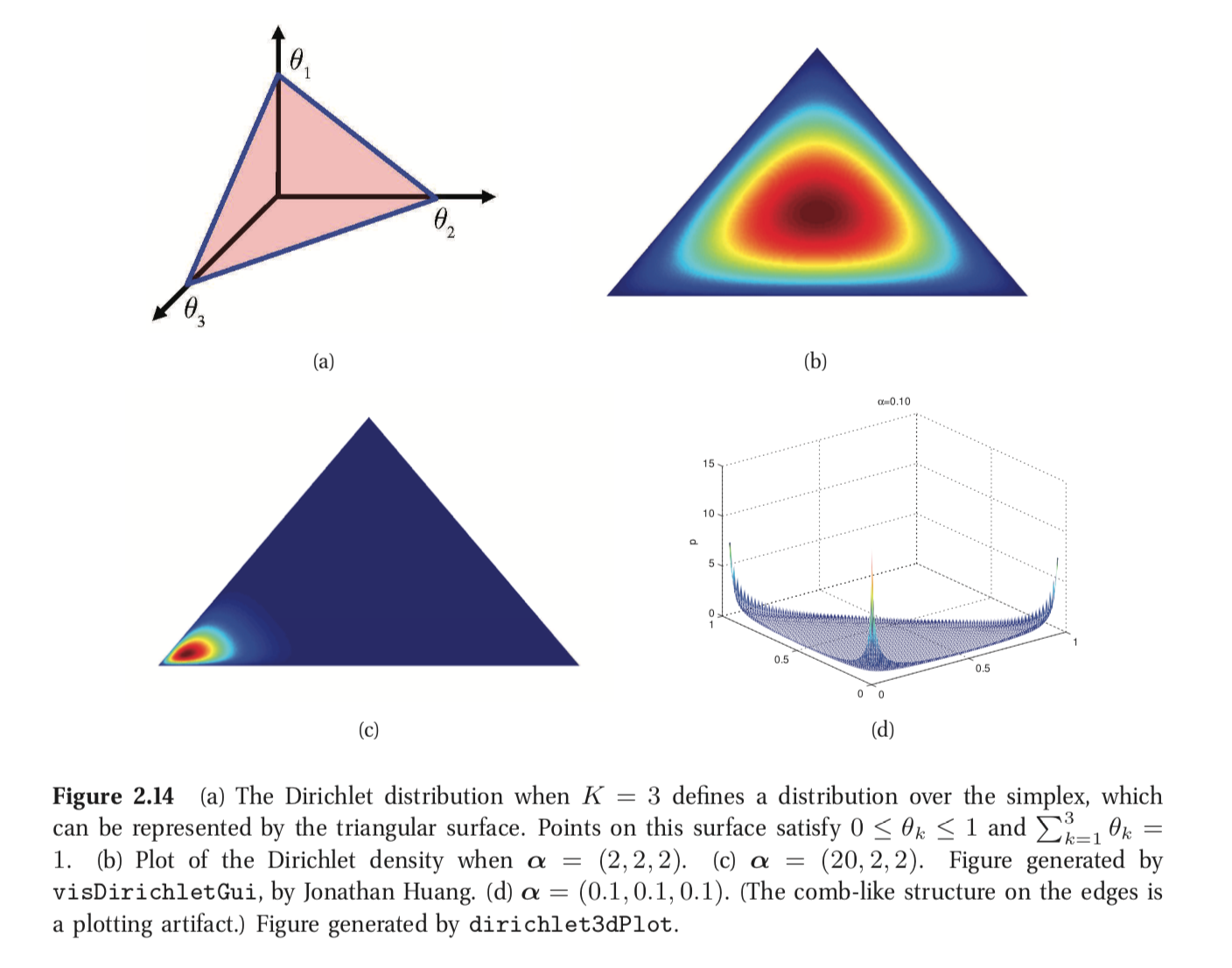
A multivariate generalization of the beta distribution is the Dirichlet distribution, which has support over the probability simplex, defined by
\[S_K=\{x:0\leq x_k\leq1, \sum_{k=1}^{K}x_k=1\}\]For example, a 2-simplex (or 2-probability-simplex) is a triangle.
The pdf is defined by:
\[Dir(x|\alpha) \triangleq \frac{1}{B(\alpha)\prod_{k=1}^{K}x_k^{\alpha_k-1}}\mathbb{I}(x\in S_K)\]where $B(\alpha) = \frac{\prod_{k=1}^{K}\Gamma(\alpha_k)}{\Gamma(\alpha_0)}$
We see that $\alpha_0 = \sum_k\alpha_k$ controls the strength of the distribution (how peaked it is), and the $\alpha_k$ control where the peak occurs. If $\alpha_k < 1$ for all k, we get “spikes” at the corner of the simplex.
2.6 Transformations of random variables
- Linear transformations
- linearity of expectation
- General transformations
- If $X$ is a discrete rv, we can derive the pmf for $y$ by simply summing up the probability mass for all the $x$’s such that $f(x) = y$:
- If $X$ is continuous, we cannot use the above Equation since $p_x(x)$ is a density, not a pmf, and we cannot sum up densities. Instead, we work with cdf’s, and write
We can derive the pdf of y by differentiating the cdf.
\[p_y(y)\triangleq\frac{d}{dy}P_y(y)=\frac{d}{dy}P_x(f^{-1}(y)) = \frac{dx}{dy}\frac{d}{dx}P_x(x)=\frac{dx}{dy}p_x(x)\]where $x=f^{-1}(y)$. Since the sign of this change is not important, we take the absolute value to get the general expression:
\[p_y(y)=\Big|\frac{dx}{dy}\Big|p_x(x)\]This is called change of variables formula.
- Central limit theorem
2.7 Monte Carlo approximation
In general, computing the distribution of a function of an rv using the change of variables formula can be difficult. One simple but powerful alternative is Monte Carlo approximation.
- First we generate $S$ samples from the distribution, call them $x_1,\cdots,x_S$. (There are many ways to generate such samples; one popular method, for high dimensional distributions, is called Markov chain Monte Carlo or MCMC; this will be explained later)
- Given the samples, we can approximate the distribution of $f(X)$ by using the empirical distribution
2.8 Information theory
Information theory is concerned with representing data in a compact fashion (a task known as data compression or source coding), as well as with transmitting and storing it in a way that is robust to errors (a task known as error correction or channel coding).
-
Entropy
The entropy of a random variable $X$ with distribution p, denoted by $\mathbb{H}(X)$ or sometimes $\mathbb{H}(p)$, is a measure of its uncertainty. In particular, for a discrete variable with $K$ states, it is defined by
\[\mathbb{H}(X) \triangleq -\sum_{k=1}^{K}p(X=k)log_2p(X=k)\] -
KL divergence
One way to measure the dissimilarity of two probability distributions, p and q, is known as the Kullback-Leibler divergence (KL divergence) or relative entropy.
\[\mathbb{KL}(p||q) \triangleq \sum_{k=1}^{K}p_k\log\frac{p_k}{q_k} \\ = \sum_k p_k \log p_k - \sum_k p_k \log q_k \\ = - \mathbb{H}(p) + \mathbb{H}(p,q)\]where $\mathbb{H}(p,q)$ is called the cross entropy, $\mathbb{H}(p,q) \triangleq -\sum_k p_k \log q_k$
$\bf{Theorem 2.8.1. :}$ (Information inequality) $\mathbb{KL} (p q) \geq 0$ with equality iff $p = q$. -
Mutual information